Showing posts with label Online Analytical Processing. Show all posts

Tuesday, 14 January 2014

What is a Factless Fact Table? Where we use Factless Fact?

We know that fact table is a collection of many facts and measures having multiple keys joined with one or more dimension tables. Facts contain both numeric and additive fields.But fact-less fact table are different from all these.
A fact-less fact table is fact table that does not contain fact. They contain only dimensional keys and it captures events that happen only at information level but not included in the calculations level, just an information about an event that happen over a period.
A fact-less fact table captures the many-to-many relationships between dimensions, but contains no numeric or textual facts. They are often used to record events or coverage information. Common examples of fact-less fact tables include:

  • Identifying product promotion events (to determine promoted products that din’t sell)
  • Tracking student attendance or registration events
  • Tracking insurance-related accident events
  • Identifying building, facility, and equipment schedules for a hospital or university

Fact-less fact tables are used for tracking a process or collecting stats. They are called so because, the fact table does not have aggregate numeric values or information.There are two types of fact-less fact tables: those that describe events, and those that describe conditions. Both may play important roles in your dimensional models.

Fact-less fact tables for Events

The first type of fact-less fact table is a table that records an event. Many event-tracking tables in dimensional data warehouses turn out to be fact-less. Sometimes there seem to be no facts associated with an important business process. Events or activities occur that you wish to track, but you find no measurements. In situations like this, build a standard transaction-grained fact table that contains no facts.
For eg.
The above fact is used to capture the leave taken by an employee.Whenever an employee takes leave a record is created with the dimensions.Using the fact FACT_LEAVE we can answer many questions like
  • Number of leaves taken by an employee
  • The type of leave an employee takes
  • Details of the employee who took leave

Fact-less fact tables for Conditions

Fact-less fact tables are also used to model conditions or other important relationships among dimensions. In these cases, there are no clear transactions or events.It is used to support negative analysis report. For example a Store that did not sell a product for a given period.  To produce such report, you need to have a fact table to capture all the possible combinations.  You can then figure out what is missing.
e.g.: fact_promo gives the information about the products which have promotions but still did not sell.
 This  fact answers the below questions:
  • To find out products that have promotions.
  • To find out products that have promotion that sell.
  • The list of products that have promotion but did not sell.
This kind of fact-less fact table is used to track conditions, coverage or eligibility.  In Kimball terminology, it is called a "coverage table."

Note:
We may have the question that why we cannot include these information in the actual fact table .The problem is that if we do so then the fact size will increase enormously .

Fact-less fact table is crucial in many complex business processes. By applying you can design a dimensional model that has no clear facts to produce more meaningful information for your business processes. Fact-less fact table itself can be used to generate the useful reports.


Monday, 13 January 2014

Different kind of FACT Tables in OBIEE

 There are basically three types of fact tables:

  • Transaction Fact Table
  • Periodic Snapshot Fact Table
  • Accumulating Snapshot Fact Table

1. Transaction Fact Tables

A transnational table is the most basic and fundamental view of the business’s operations These fact tables represent an event that occurred at an instantaneous point in time. A row exists in the fact table for a given customer or product only if a transaction event occurred. Conversely, a given customer or product likely is linked to multiple rows in the fact table because hopefully the customer or product is involved in more than one transaction. Transaction data often is structured quite easily into a dimensional framework. The lowest-level data is the most naturally dimensional data, supporting analyses that cannot be done on summarized data. Unfortunately, even with transaction-level data, there is still a whole class of urgent business questions that are impractical to answer using only transaction detail.

2. Periodic Snapshot Fact Tables

Periodic snapshots are needed to see the cumulative performance of the business at regular, predictable time intervals. Unlike the transaction fact table, where we load a row for each event occurrence, with the periodic snapshot, we take a picture (hence the snapshot terminology) of the activity at the end of a day, week, or month, then another picture at the end of the next period, and so on. Eg: A performance summary of a salesman over the previous month .

The periodic snapshots are stacked consecutively into the fact table. The periodic snapshot fact table often is the only place to easily retrieve a regular, predictable, trendable view of the key business performance metrics.Periodic snapshots typically are more complex than individual transactions.
Advantages:When transactions equate to little pieces of revenue, we can move easily from individual transactions to a daily snapshot merely by adding up the transactions, such as with the invoice fact tables from this chapter. In this situation, the periodic snapshot represents an aggregation of the transactional activity that
occurred during a time period. We probably would build the daily snapshot only if we needed a summary table for performance reasons.

Where to use Snapshots?
When you use your credit card, you are generating transactions, but the credit card issuer’s primary source of customer revenue occurs when fees or charges are assessed. In this situation, we can’t rely on transactions alone to analyze revenue performance. Not only would crawling through the transactions be time-consuming, but also the logic required to interpret the effect of different kinds of transactions on revenue or profit can be horrendously complicated. The periodic snapshot again comes to the rescue to provide management with a quick, flexible view of revenue. 

3. Accumulating Snapshot Fact Tables

This type of fact table is used to show the activity of a process that has a well-defined beginning and end, e.g., the processing of an order. An order moves through specific steps until it is fully processed. As steps towards fulfilling the order are completed, the associated row in the fact table is updated.
Accumulating snapshots almost always have multiple date stamps, representing the predictable major events or phases that take place during the course of a lifetime. Often there’s an additional date column that indicates when the snapshot row was last updated. Since many of these dates are not known when the fact row is first loaded, we must use surrogate date keys to handle undefined dates.
In sharp contrast to the other fact table types, we purposely revisit accumulating snapshot fact table rows to update them. Unlike the periodic snapshot, where we hang onto the prior snapshot, the accumulating snapshot merely reflects the accumulated status and metrics. Sometimes accumulating and periodic snapshots work in conjunction with one another

Types of Facts in Data Warehousing

A fact table is the central table in a star schema of a data warehouse. A fact table stores quantitative information for analysis and is often denormalized form.

A fact table works with dimension tables. A fact table holds the data to be analyzed, and a dimension table stores data about the ways in which the data in the fact table can be analyzed.
Thus, fact tables typically has two types of columns, foreign keys to dimension tables and measures those that contain numeric facts. A fact table can contain fact’s data on detail or aggregated level.
Eg: Sales, Cost, Profit, and many more.

Types of Facts

  • Non-Additive
  • Semi-Additive
  • Additive

Additive
Additive facts are facts that can be summed up through all of the dimensions in the fact table.
Eg: Sales fact.

Semi-Additive
Semi-additive facts are facts that can be summed up for some of the dimensions in the fact table, but not the others.
Eg: Daily balances fact can be summed up through the customers dimension but not through the time dimension.

Non-Additive
Non-additive facts are facts that cannot be summed up for any of the dimensions present in the fact table.
Eg: Facts which have percentages, Ratios calculated.

Wednesday, 8 January 2014

Oracle Data Integrator 11.1.1.7.0 (ODI) Step By Step Installation On Windows 7 x86_64-Bit

Prerequisites

  • You must use the 64-bit version of JDK or JRockit to install on 64-bit machines. On Windows, the location of the JDK must be on the same drive as the installers.
  • In the previous post I have posted the steps RCU installation for Oracle Data Integration for 11.1.1.7.0 verson. We can take this as a continuation of that post. Please follow all the prerequisites before going to ODI 11g installation.
  • One Application Server.
Download the ODI 11g (11.1.1.7.0) from Oracle eDelivery or from the below link:


If you have not done already, please download ODI 11g installation files. Please make sure all the zipped files have downloaded correctly and unzipped into a single folder. Make sure that, no spaces are there in the folder path where setup files are located.

To start the installer, go to the directory where you unpacked the archive file and switch to the Disk1 directory.
cd unpacked_archive_directory\Disk1                  
setup.exe -jreLoc JRE_LOCATION                      

The installer requires the full path to the location of a Java Runtime Environment (JRE) on your system, which must be specified using the -jreLoc parameter.

My java is installed on C:\Java path, so here is the command to start the ODI installer..
Note:
  • If you installed Oracle WebLogic Server, a JRE was installed on your system in the jdk_version directory inside the Middleware home. You can use this location as the JRE_LOCATION to start the installer.
  • If you are using IBM WebSphere as your Application Server, you must provide the full path to a certified JRE installed on your system.
Step 1. Oracle Universal Installer will start the OBIEE 11g setup screen.

Click 'Next' with the below Welcome screen.

Step 2.  Select the method you want to use for obtaining software updates, or select Skip Software Updates if you do not want to get updates.
If updates are found, the installer will automatically apply them at this point. Some updates will require the installer to automatically be restarted; if this happens, the Install Software Updates screen will not be seen the next time.


Step 3. The Oracle Data Integrator installer provides the following installation options; you can select any combination of these options during the installation:
  • Developer Installation: 
This installation includes the ODI Studio and the Oracle Data Integrator Software Development Kit (SDK).
Note that this installation does not include the Standalone Agent or the scripts for managing sessions or scenarios from the command line. If a Standalone Agent will be needed, select Standalone Installation in addition to Developer Installation.
  • Standalone Installation:
This installation includes an Oracle Data Integrator standalone agent.
  • Java EE Installation:
This installation includes the Java EE agent, Oracle Data Integrator Console, and Public Web Services.
Here, i have selected all the components except ODI Standalone Agent.

Step 4. The installer checks for system prerequisites such as operating system certification, recommended operating system packages, and physical memory. If there is a problem, a short error message appears and you will have an opportunity to correct the issue before continuing the installation.

Step 5. This screen allows you to specify the absolute path for the Oracle home location.

NOTE - The specified Oracle home directory must be an empty directory or an existing Oracle Data Integrator home location.

If you selected Java EE Installation on the Select Installation Type screen, you will also be asked to provide the location of your Middleware home.

I have installed Weblogic already on my machine that comes with OBIEE. So, I'm giving here "OBIEE Middleware" location as "Oracle Middleware Home".

It will automatically populate the Oracle Home Directory as Oracle_OD1 within that Middleware Home location.


Step 6. Select the application server you want to use for your Java EE components.
As I have installed OBIEE 11.1.1.7.0, I used the Weblogic server as my Application Server.

Step 7. This screen allows you to select whether you want to configure the Oracle Data Integrator Studio and the Standalone Agent with an existing Master and Work Repository pair.
  • Configure Repositories:
This option creates a connection to a work repository for the Oracle Data Integrator Studio. It also configures the odiparams file for the Standalone Agent to connect the master repository. The agent definition is declared in the topology and corresponding agent startup scripts and shortcuts are created. With this configuration, the standalone agent can be started with no additional configuration.
Select this option if you have existing 11g Master and Work Repositories. 
  •  Skip Repository Configuration:
Select this option to continue with the Oracle Data Integrator installation without configuring the repositories. Once installed, you can use the Oracle Data Integrator Studio JDev Gallery to create or configure the repositories.
NOTE: Select Skip Repository Configuration if:
  • Your database is not supported by Oracle's Repository Creation Utility (RCU). You will need to configure these components manually after the installation. For more information see Appendix E, "Creating Repositories with Oracle Data Integrator Studio".
  • Your schemas have not yet been upgraded to the latest release.
If you have already done with the RCU Installation for ODI, select Configure Repositories.

Step 8. This screen allows you to specify the connection string to the database that hosts the Master Repository and the database user name and password.


Step 9. This screen allows you to specify the password for the Supervisor user. This is the same password specified on the Custom Variables screen when you ran RCU to create the schemas.

Displays the ODI username with Supervisor privileges. This field cannot be edited.

Note that the user name is SUPERVISOR (all CAPS) and ODI user names are case-sensitive. When you are asked to provide the Supervisor name later (for example, in ODI Studio), you must enter the name exactly at it appears here (SUPERVISOR), in all CAPS.


Step 10. This screen allows you to select an existing Work Repository from the list.

Step 11. This screen allows you to verify the installation options you selected. Click Install to begin the installation.

Step 12. This screen allows you to see the progress of the installation.

Step 13. This screen allows you to see the progress of any post-installation configuration tasks you may have selected.

Step 14. Click Save to save your configuration information to a file. This information includes port numbers, installation directories, disk space usage, URLs, and component names which you may need to access at a later time.
After saving your configuration information, click Finish to dismiss the installer.

Monday, 6 January 2014

Oracle Data Integrator 11.1.1.7.0 (ODI) RCU Installation

Installing a Database

Oracle Data Integrator stores information in a repository that is stored in a database schema. The Repository Creation Utility (RCU) is able to create the schema and the repository in the database. RCU supports Oracle, Microsoft SQL Server and IBM DB2 databases and supports the installation of a Master Repository and Work Repositories into a single schema.

If you have installed database already on your system, you can simply skip this section.

Before we starting the installation of RCU, we need to choose that which database we are going to use in our application. Here I am giving how to run RCU in Oracle database on our local machine. It is good to install Oracle Database Enterprise Edition to take full advantage of database for data types like spatial data or features like OLAP.

Prerequisites:

Here I am giving the installation steps that how I have installed RCU in my windows 32bit Operating system. If you have 64 bit OS, no worry the steps are same.

    Minimum of 4GB RAM required, 3 GB RAM would work but, system would be slow.

    Minimum of 10GB hard disk memory required.

    Do not use any directory name with space while installing/working with Oracle DB and OBIEE 11g.

Using RCU to Create the Database Schema

Oracle Data Integration 11g (11.1.1.7.0) is now standardized with Oracle Fusion Middleware and hence leverage database for metadata storage just like any other middleware product. So here we are going to install ODI 11g metadata schema on oracle database you just installed and configured. Same process can be leveraged to install metadata schema on other supported databases as well.
If you have not done already, please download RCU installation files from below URL:


Locate Required Additional Software's:

Please make sure all the zipped files have downloaded correctly and unzipped into a single folder and no any spaces in the folder path where setup files are located..

Now we will start the installation of metadata schema using Repository Creation Utility (RCU).

From unzipped folder for RCU, run rcu.bat file to start the Repository Creation Utility: 
For this practice, rcu.bat file is located under E:\Softwares\ODI\rcuHome\BIN directory.

Step 1. RCU utility will launch the GUI based wizard to guide you through the steps. Click Next to continue.

Step 2. Select Create from the below screen and click Next.

Step 3. In the below step Make sure database type is Oracle Database and enter following information to continue.

Step 3.1. Since we are using oracle database, RCU will show a warning message that you can just ignore and can continue the installation.

Step 3.2. Click OK to continue once RCU validates and initializes database configuration.

Step 4. In the next step it will ask for the prefix to create the metadata schema. By default, it is showing 'DEV'. If we want to change the prefix we can  change it. From the below window select appropriate schema which we need to install. I have selected only two which is showing in the screenshot.

Step 5. Click 'Next' from the above screen to create schema and the click 'OK' once RCU shows schema creation prerequisites check completed.

Step 6. In the next step, Enter password for both the schema as you like with the password conditions (such as alphabet, numeric and with special character) and click 'Next' to continue.

Step 7. On the Custom Variables screen, provide the following information as described as follows,
Master Repository ID: A specific ID for the new Master Repository. Master Repository ID values must be between 0 and 899. Default value is 001.

Supervisor Password: Password of the Supervisor user. You must confirm this password on the following line.

Work Repository Type:
Specify how the Work Repository will be used:
  • Use Development (D) for creating a development repository. This type of repository allows management of design-time objects such as data models and projects (including interfaces, procedures, etc.) A development repository also includes the run-time objects (scenarios and sessions). This type of repository is suitable for development environments.
D is the default work repository type.
  • Use Execution (E) for creating an execution repository: This type of repository only includes run-time objects (scenarios, schedules and sessions). It allows launching and monitoring of data integration jobs in Operator Navigator. Such a repository cannot contain any design-time artifacts. Designer Navigator cannot be used with it. An execution repository is suitable for production environments. 
Work Repository ID: A specific ID for the new Work Repository. Default value is 001.

Work Repository Name: A unique name for the Work Repository. Default is WORKREP.

Work Repository Password: Provide a password for the Work Repository.

Step 8. Click 'Next' with the above step to have RCU create the selected schema.

Step 8.1. Click 'OK' to continue creation of tablespace.

Step 8.2. Once tablespace created, click 'OK' to continue.

Step 9. Now RCU will create required schema objects within the tablespace just created. So Click 'Create' with next step and continue.

Step 10. Click 'Close' to finish RCU wizard once schema are created successfully.

 With the above step the installation of RCU is completed.

Note:
Remember the password which we have given for all the users/schema so far and we will continue to use the same password. We will need this password for ODI installation as well to let ODI installer knows where the metadata schema located and what is the password to connect to the schema. Now we can log-in to the oracle database and can whether this schema (DEV_ODI_REPO) is available.


Tuesday, 17 September 2013

What is an OLAP and Explain OLAP's advantages with example?

OLAP (or Online Analytical Processing) has been growing in popularity due to the increase in data volumes and the recognition of the business value of analytics. It uses database tables (fact and dimension tables) to enable multidimensional viewing, analysis and querying of large amounts of data. E.g. OLAP technology could provide management with fast answers to complex queries on their operational data or enable them to analyze their company's historical data for trends and patterns.

OLAP allows business users to slice and dice data at will. Normally data in an organization is distributed in multiple data sources and are incompatible with each other. A retail example: Point-of-sales data and sales made via call-center or the Web are stored in different location and formats. It would a time consuming process for an executive to obtain OLAP reports such as - What are the most popular products purchased by customers between the ages 15 to 30?

Part of the OLAP implementation process involves extracting data from the various data repositories and making them compatible. Making data compatible involves ensuring that the meaning of the data in one repository matches all other repositories. An example of incompatible data: Customer ages can be stored as birth date for purchases made over the web and stored as age categories (i.e. between 15 and 30) for in store sales.The major OLAP vendors are Hyperion, Cognos, Business Objects, MicroStrategy.
OLAPs are designed to give an overview analysis of what happened. Hence the data storage (i.e. data modeling) has to be set up differently. The most common method is called the star design.


The central table in an OLAP start data model is called the fact table. The surrounding tables are called the dimensions. Using the above data model, it is possible to build reports that answer questions such as:

  • The supervisor that gave the most discounts.
  • The quantity shipped on a particular date, month, year or quarter.
  • In which pincode did product A sell the most.

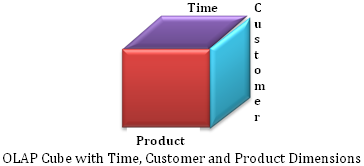
To obtain answers, such as the ones above, from a data model OLAP cubes are created. OLAP cubes are not strictly cuboids - it is the name given to the process of linking data from the different dimensions. The cubes can be developed along business units such as sales or marketing.Or a giant cube can be formed with all the dimensions.

OLAP can be a valuable and rewarding business tool. Aside from producing reports, OLAP analysis can aid an organization evaluate balanced scorecard targets.

Business intelligence refers to computer-based methods for identifying and extracting useful information from business data. OLAP (online analytical processing) as the name suggest is a compilation of ways to query multi-dimensional databases.

OLAP is a class of systems, which provide answers to multi-dimensional queries.Typically OLAP is used for marketing, budgeting, forecasting and similar applications. It goes without saying that the databases used for OLAP are configured for complex and ad-hoc queries with a quick performance in mind. Typically a matrix is used to display the output of an OLAP. The rows and columns are formed by the dimensions of the query. They often use methods of aggregation on multiple tables to obtain summaries.For example,it can be used to find out about the sales of this year in Wal-Mart compared to last year? What is the prediction on the sales in the next quarter? What can be said about the trend by looking at the percentage change?
OLAP tools provides multidimensional data analysis and they provide summaries of the data but contrastingly, data mining focuses on ratios, patterns and influences in the set of data.